The openGUTS Matlab version

Table of contents

About
BLOCK 1. Initial things
BLOCK 2. Calibration
BLOCK 3. Predictions: LCx versus time
BLOCK 4. Validation: comparison to new data
BLOCK 5. Predictions: LPx
BLOCK 6. Batch predictions for LPx
BLOCK 7. Demonstration of predictions for test design

About

Main script for the openGUTS Matlab version. This version started as the prototype for the standalone openGUTS software (the latter developed by WSC). This programme follows the workflow as laid down in the 2018 EFSA Scientific Opinion on TKTD modelling:

Calibration: load one or more data sets from file using the Matlab input GUI. The input data set will be shown in a plot, and calibration of GUTS-RED-SD and GUTS-RED-IT will commence automatically. Fitting results will be shown on screen.
Validation: load one or more data sets from file using the Matlab input GUI. The results from the calibration will be used to predict the survival probability for the exposure scenarios in the validation data sets. Results will be shown on screen.
Prediction: load one or more exposure profiles from file using the Matlab input GUI. The results from the calibration will be used to predict the survival probability for the exposure scenarios in the exposure profiles. Results will be shown on screen.

Input files for survival data and exposure profiles are read from the respective folders [input_data] and [input_profile]. Information from the calibration is saved into the folder [output_sample]. Figures and log files for the output can be found in the folder [output_report].

Author: Tjalling Jager (DEBtox Research)
Date: December 2019
Web support: http://www.openguts.info
Funding: Cefic-LRI, see http://debtox.nl/projects/project_guts2.html

% =========================================================================
% Copyright (c) 2018-2019, Tjalling Jager (tjalling@debtox.nl).
% This file is part of the Matlab version of openGUTS.
%
% This program is free software: you can redistribute it and/or modify it
% under the terms of the GNU General Public License as published by the
% Free Software Foundation, either version 3 of the License, or (at your
% option) any later version.
%
% This program is distributed in the hope that it will be useful, but
% WITHOUT ANY WARRANTY; without even the implied warranty of
% MERCHANTABILITY or FITNESS FOR A PARTICULAR PURPOSE. See the GNU General
% Public License for more details.
%
% You should have received a copy of the GNU General Public License along
% with this program. If not, see <https://www.gnu.org/licenses/>.
% =========================================================================

BLOCK 1. Initial things

The helper function [pathdefine] makes sure that the [engine] folder (which holds the actual functions that perform the calculations) is in the Matlab path. The script [initial_setup] takes care of some general setting up. In this block, you can set a name for the analysis (used for identifying output files), and set a switch to use a saved sample from a previous calibration rather than loading a file and calibrating it.

pathdefine    % places the [engine] folder in Matlab search path
initial_setup % calls a script that sets things up

% rng(2.2) % seed the random number generator with a specific value (this overrides the shuffle in the [initial_setup])
% % Fixing the seed is helpful for testing: it ensures that every run of this file will be exactly the same.

% Provide a name for the study to be used for the plots and saved files.
GLO.basenm       = 'propiconazole'; % name used for identifying the analysis
use_saved_sample = 0; % when set to 1, use saved calibration file rather than make a new calibration
GLO.fix_hb_cal   = 1; % when set to 1, fit [hb] to the control data for all calibration data sets, and keep fixed
% Note: for the validation data set, there is a separate switch for fixing [hb] in BLOCK 4.
GLO.intermed_plots = 0; % when set to 1, makes intermediate plots of parameter space to monitor progress

BLOCK 2. Calibration

Based on the setting of [use_saved_sample], a saved calibration is shown (regenerated from the project MAT file) or a new calibarion is performed. The calibration function [calc_optim] can be used for both purposes. The Matlab GUI [uigetfile] is used to select files.

Note: the second and third input arguments for [calc_optim] are a switch for SD/IT (1/2) and a flag for optimisation (1) or show saved optimisation (2). The [plot_main] also has flags for SD/IT (1/2), and a second argument, which is a vector of two flags: for the stage of the analysis we are in, and for whether to plot model curves or not.

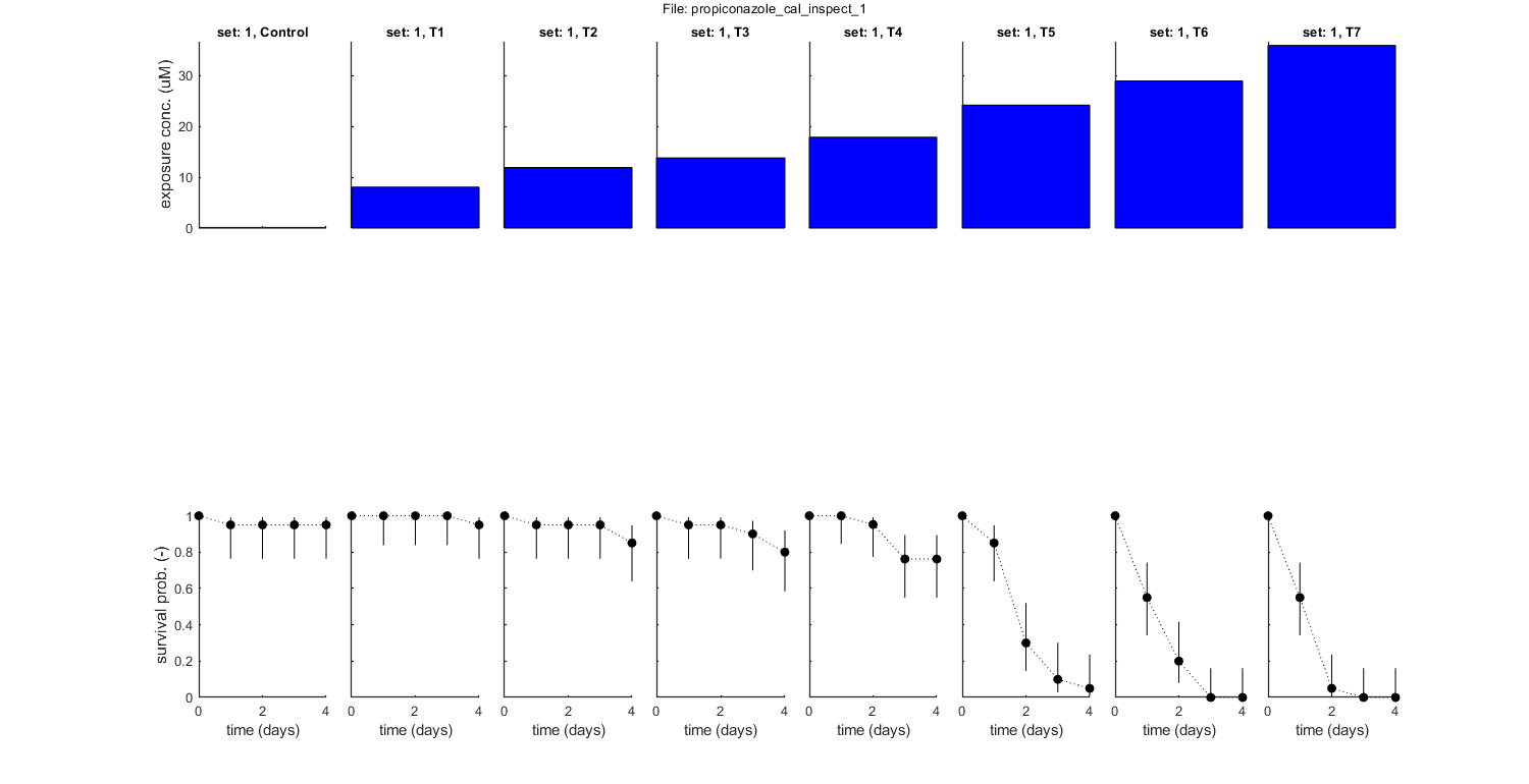
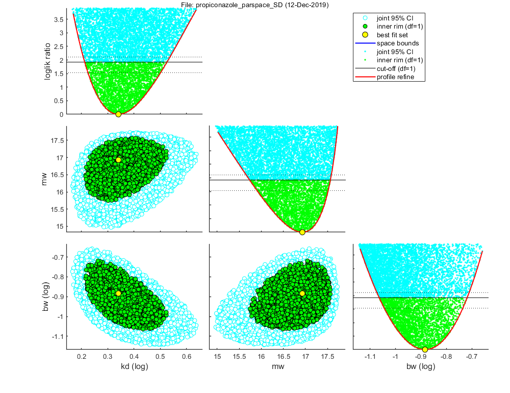
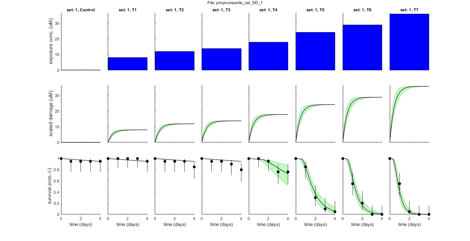
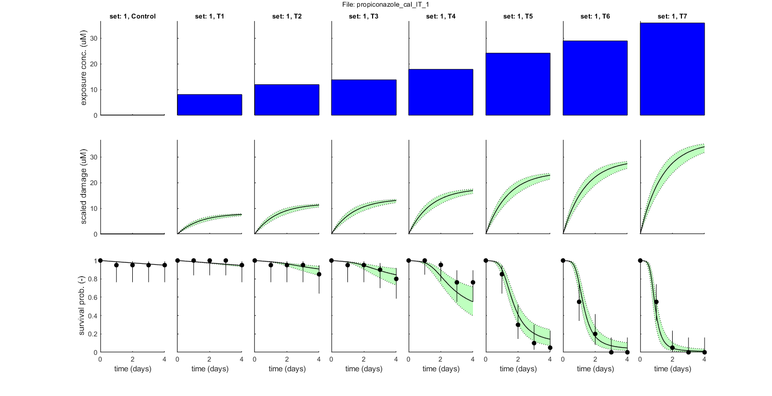
if use_saved_sample == 1
    % BLOCK 2.1. Use saved calibration results.
    % Note: Optimised parameter values and sample for confidence region
    % will be read from a saved MAT file (selected by the Matlab GUI).
    % Therefore, there is no need for calibration (as long as the saved
    % file exists).
    %
    % Note: Calling [calc_optim] to show saved optimisation makes [DATAcal]
    % from the saved set global, as well as [GLO.basenm], [GLO.concunit]
    % and [GLO.fix_hb_cal]. These are all associated with the previous
    % calibration, so they should not be changed after calibration has been
    % performed.

    filename = uigetfile('output_sample/*.mat','Select a saved project file (selecting either SD or IT will use both)','MultiSelect','off'); % use Matlab GUI to select MAT file
    if ~iscell(filename) && numel(filename) == 1 && filename(1) == 0 % if cancel is pressed ...
        return % simply stop
    end
    GLO.basenm = filename(1:end-16); % remove the last part (_parspace_SD.mat) of the filename so that the basename remains
    % First, see if there is an output folder for this specific studyname, and otherwise create it.
    savestr = ['output_report',filesep,GLO.basenm];
    if ~exist(savestr,'dir')
        mkdir(savestr); % if not, create it
    end

    % Use [calc_optim] to recreate the plot of parameters space and [plot_main] to plot the fit (standard plot).
    calc_optim([],1,2); % SD just use saved set, without new optimisation
    calc_optim([],2,2); % IT just use saved set, without new optimisation
    plot_main(DATAcal,2,[1 1]) % IT plot of calibration data with the fit (stage 1, plot model on)
    plot_main(DATAcal,1,[1 1]) % SD plot of calibration data with the fit (stage 1, plot model on)

else
    % BLOCK 2.2. Load and prepare calibration data.
    % The data set will be loaded and translated to the internal
    % representation, which is returned in [DATAcal]. [DATAcal] is made
    % global (in [initial_setup]) as it is called many times during
    % optimisation.

    [filename,filepath] = uigetfile('input_data/*.txt','Select file(s) for calibration','MultiSelect','on'); % use Matlab GUI to select file(s)
    if ~iscell(filename) && numel(filename) == 1 && filename(1) == 0 % if cancel is pressed ...
        return % simply stop
    end

    [DATAcal,error_flag] = load_data(filename,filepath,1); % load and prepare the data set for stage 1 (returned as structured cell array, so [data_all] can include multiple data sets)
    if error_flag == 1 % see if there are errors spotted in the input file
        return % simply return (stop and do nothing)
    end
    plot_main(DATAcal,[],[1 0]) % inspection plot of data (stage 1, plot model off)
    % Note: the 1 in the calls above signal that we are loading, preparing
    % and plotting data for stage 1: calibrations.

    % BLOCK 2.3. Ranges for the model parameters. Note: the parameter
    % structure [pmat] will be automatically generated by [startgrid]
    % below. Experts can make changes to the [pmat] after that.
    %
    % WARNING: some settings of [pmat] will lead to poor performance or
    % even complete failure of the calibration algorithm. Therefore, when
    % messing with this matrix, expertise and care are essential to get
    % reliable results.

    % Make separate parameter matrices for SD and IT.
    pmat_SD = startgrid(1); % create reasonable SD parameter ranges from the data set
    pmat_IT = startgrid(2); % create reasonable IT parameter ranges from the data set
    % Below this line, modifications to the parameter matrices can be inserted.

    % BLOCK 2.4. Perform calibration.
    % Note that the starting values in [pmat] are only used for fixed
    % parameters in the analysis; for fitted parameter, only the ranges and
    % other settings are used. [calc_optim] finds the global optimum,
    % confidence intervals on parameters, and the joint confidence region
    % (to be used for predictions). The sample is saved in a MAT file with
    % an extension indicating the analysis (SD or IT), which is
    % automatically used by the post-analyses.

    % Use [calc_optim] to perform the calibration and [plot_main] to plot the fit (standard plot).
    calc_optim(pmat_SD,1,1); % SD, new optimisation
    calc_optim(pmat_IT,2,1); % IT, new optimisation
    plot_main(DATAcal,1,[1 1]) % SD plot of calibration data with the fit (stage 1, plot model on)
    plot_main(DATAcal,2,[1 1]) % IT plot of calibration data with the fit (stage 1, plot model on)

end

% return % the return stops the analysis, so we can run this script in parts

Following data sets are loaded for calibration:
    set: 1, file: propiconazole_constant.txt

 
Settings for parameter search ranges:
=====================================================================
kd    bounds:   0.001641 -      143.8 1/d      fit: 1 (log)
mw    bounds:   0.002202 -      35.56 uM       fit: 1 (norm)
hb    bounds:    0.01307 -    0.01307 1/d      fit: 0 (norm)
bw    bounds:  0.0007332 -       9310 1/(uM d) fit: 1 (log)
Fs    bounds:          1 -          1 [-]      fit: 0 (norm)
=====================================================================
Special case: stochastic death (SD) 
Background hazard rate fixed to a value fitted on controls
 
Starting round 1 with initial grid of 2016 parameter sets
  Status: best fit so far is (minloglik) 131.8625
Starting round 2, refining a selection of 200 parameter sets, with 60 tries each
  Status: 15 sets within total CI and 6 within inner. Best fit: 125.8154
Starting round 3, refining a selection of 200 parameter sets, with 40 tries each
  Status: 275 sets within total CI and 118 within inner. Best fit: 125.8154
Starting round 4, refining a selection of 747 parameter sets, with 60 tries each
  Status: 7851 sets within total CI and 2750 within inner. Best fit: 125.8154
  Finished sampling, running a simplex optimisation ...
  Status: 7852 sets within total CI and 2751 within inner. Best fit: 125.8153
Starting round 5, creating the profile likelihoods for each parameter
  Finished profiling, running a simplex optimisation on the best fit set found ...
  Status: 7853 sets within total CI and 2752 within inner. Best fit: 125.8153

 
=================================================================================
Results of the parameter estimation
=================================================================================
   openGUTS Matlab: v1.0 (10 December 2019)
   Base name      : propiconazole 
   Analysis date  : 12-Dec-2019 (17:12) 
   Following data sets are loaded for calibration:
     set: 1, file: propiconazole_constant.txt
   Sample: 7853 sets in joint CI and 2752 in inner CI.
   Propagation set: 1226 sets will be used for error propagation.
   Minus log-likelihood has reached 125.82 (AIC=257.63). 
Best estimates and 95% CIs on single parameters
==========================================================================
kd    best:      2.191 (     1.630  -     3.353 ) 1/d       fit: 1 (log)
mw    best:      16.93 (     15.74  -     17.57 ) uM        fit: 1 (norm)
hb    best:    0.01307 (       NaN  -       NaN ) 1/d       fit: 0 (norm)
bw    best:     0.1306 (   0.08627  -    0.1912 ) 1/(uM d)  fit: 1 (log)
Fs    best:          1 (       NaN  -       NaN ) [-]       fit: 0 (norm)
==========================================================================
Special case: stochastic death (SD) 
Background hazard rate fixed to a value fitted on controls
 
Extra information from the fit:
==========================================================================
Depuration/repair time (DRT95)    : 1.37 (0.893 - 1.84) days 
Parameter ranges used for the optimisation:
kd    range:   0.001641 -      143.8 
mw    range:   0.002202 -      35.56 
hb    range:    0.01307 -    0.01307 
bw    range:  0.0007332 -       9310 
Fs    range:          1 -          1 
==========================================================================
Time required for optimisation: 18.2 secs
 
 
Settings for parameter search ranges:
=====================================================================
kd    bounds:   0.001641 -      143.8 1/d      fit: 1 (log)
mw    bounds:   0.002202 -      71.85 uM       fit: 1 (norm)
hb    bounds:    0.01307 -    0.01307 1/d      fit: 0 (norm)
bw    bounds:        Inf -        Inf 1/(uM d) fit: 0 (norm)
Fs    bounds:       1.05 -         20 [-]      fit: 1 (log)
=====================================================================
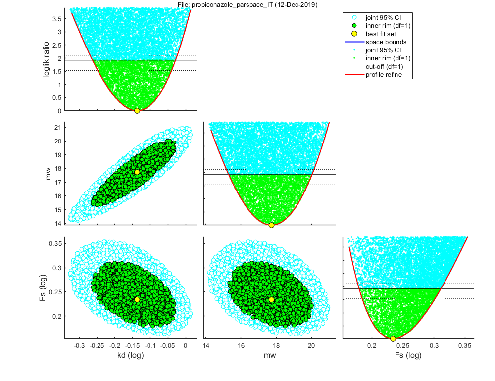
Special case: individual tolerance (IT) 
Background hazard rate fixed to a value fitted on controls
 
Starting round 1 with initial grid of 2016 parameter sets
  Status: best fit so far is (minloglik) 131.3463
Starting round 2, refining a selection of 200 parameter sets, with 60 tries each
  Status: 19 sets within total CI and 7 within inner. Best fit: 127.9601
Starting round 3, refining a selection of 200 parameter sets, with 40 tries each
  Status: 383 sets within total CI and 123 within inner. Best fit: 127.9595
Starting round 4, refining a selection of 914 parameter sets, with 54 tries each
  Status: 8885 sets within total CI and 3038 within inner. Best fit: 127.9594
  Finished sampling, running a simplex optimisation ...
  Status: 8885 sets within total CI and 3039 within inner. Best fit: 127.9593
Starting round 5, creating the profile likelihoods for each parameter
  Finished profiling, running a simplex optimisation on the best fit set found ...
  Status: 8886 sets within total CI and 3040 within inner. Best fit: 127.9593

 
=================================================================================
Results of the parameter estimation
=================================================================================
   openGUTS Matlab: v1.0 (10 December 2019)
   Base name      : propiconazole 
   Analysis date  : 12-Dec-2019 (17:12) 
   Following data sets are loaded for calibration:
     set: 1, file: propiconazole_constant.txt
   Sample: 8886 sets in joint CI and 3040 in inner CI.
   Propagation set: 1374 sets will be used for error propagation.
   Minus log-likelihood has reached 127.96 (AIC=261.92). 
Best estimates and 95% CIs on single parameters
==========================================================================
kd    best:     0.7292 (    0.5458  -    0.9359 ) 1/d       fit: 1 (log)
mw    best:      17.73 (     15.30  -     20.03 ) uM        fit: 1 (norm)
hb    best:    0.01307 (       NaN  -       NaN ) 1/d       fit: 0 (norm)
bw    best:        Inf (       NaN  -       NaN ) 1/(uM d)  fit: 0 (norm)
Fs    best:      1.714 (     1.511  -     2.047 ) [-]       fit: 1 (log)
==========================================================================
Special case: individual tolerance (IT) 
Background hazard rate fixed to a value fitted on controls
 
Extra information from the fit:
==========================================================================
Beta of the threshold distribution: 6.80 (5.11 - 8.88) (-) 
Depuration/repair time (DRT95)    : 4.11 (3.20 - 5.49) days 
Parameter ranges used for the optimisation:
kd    range:   0.001641 -      143.8 
mw    range:   0.002202 -      71.85 
hb    range:    0.01307 -    0.01307 
bw    range:        Inf -        Inf 
Fs    range:       1.05 -         20 
==========================================================================
Time required for optimisation: 23.4 secs

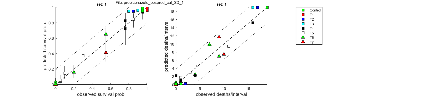
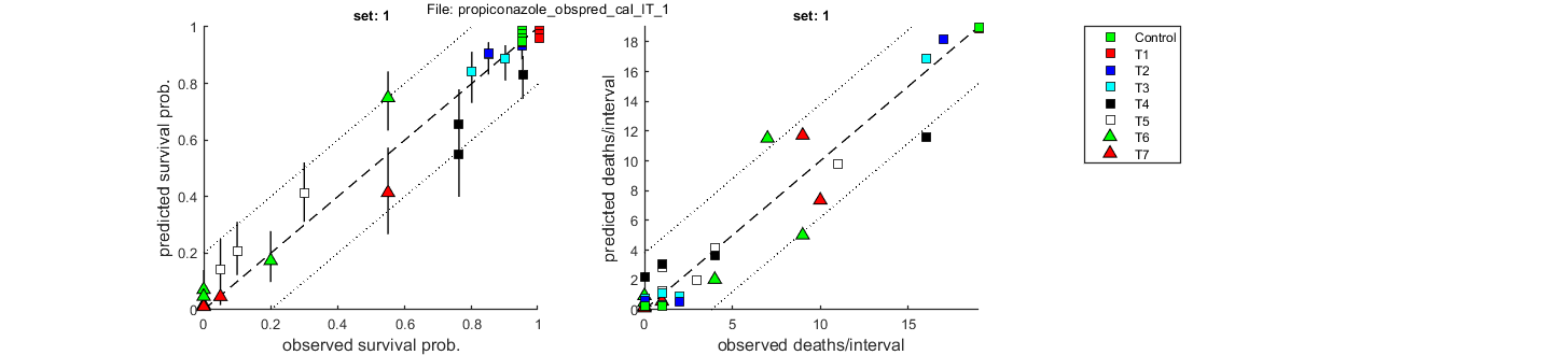
Goodness of fit measures for calibration
  Special case: stochastic death (SD)
=====================================================================
Model efficiency (NSE, r-square)          : 0.9811 
Normalised root-means-square error (NRMSE): 7.948 % 
Survival probability prediction error (SPPE) for each treatment
     Data set     treatment    value
        1         Control     +0.0937 % 
        1              T1     +0.0937 % 
        1              T2     -9.91 % 
        1              T3     -14.9 % 
        1              T4     +3.79 % 
        1              T5     -0.558 % 
        1              T6     -0.690 % 
        1              T7     -0.0297 % 
=====================================================================
Warning: these measures need to be interpreted more qualitatively
  as they, strictly speaking, do not apply to quantal data

Goodness of fit measures for calibration
  Special case: individual tolerance (IT)
=====================================================================
Model efficiency (NSE, r-square)          : 0.9605 
Normalised root-means-square error (NRMSE): 11.665 % 
Survival probability prediction error (SPPE) for each treatment
     Data set     treatment    value
        1         Control     +0.0937 % 
        1              T1     +0.395 % 
        1              T2     -5.77 % 
        1              T3     -4.40 % 
        1              T4     +21.1 % 
        1              T5     -9.25 % 
        1              T6     -4.71 % 
        1              T7     -1.12 % 
=====================================================================
Warning: these measures need to be interpreted more qualitatively
  as they, strictly speaking, do not apply to quantal data

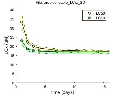
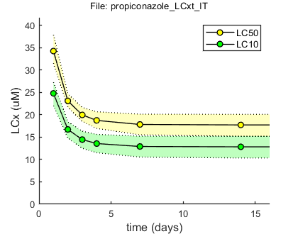
BLOCK 3. Predictions: LCx versus time

LCx,t values are calculated for several effect percentages and several preset time points (defined in [initial_setup]). Optimised parameter values and sample to create CIs will be read from the saved MAT file.

calc_lcx(16,1); % SD, calculate LCx values with CI (final timepoint t=16)
calc_lcx(16,2); % IT, calculate LCx values with CI (final timepoint t=16)

% return % the return stops the analysis, so we can run this script in parts

Results table for LCx,t (uM), with 95% CI
  Special case: stochastic death (SD)
======================================================================
time (d)       LC50               LC20               LC10               
======================================================================
   1   33.3 ( 29.9 -  37.7)  25.5 ( 23.1 -  28.0)  23.1 ( 20.8 -  25.2) 
   2   22.6 ( 21.5 -  24.0)  19.5 ( 18.5 -  20.3)  18.6 ( 17.5 -  19.2) 
   3   20.1 ( 19.2 -  21.0)  18.2 ( 17.2 -  18.8)  17.7 ( 16.6 -  18.2) 
   4   19.0 ( 18.1 -  19.8)  17.7 ( 16.7 -  18.3)  17.4 ( 16.2 -  18.0) 
   7   17.9 ( 16.9 -  18.6)  17.3 ( 16.1 -  17.9)  17.1 ( 15.9 -  17.7) 
  14   17.4 ( 16.2 -  18.0)  17.1 ( 15.9 -  17.7)  17.0 ( 15.8 -  17.6) 
  21   17.2 ( 16.0 -  17.9)  17.0 ( 15.8 -  17.7)  17.0 ( 15.7 -  17.6) 
  28   17.1 ( 15.9 -  17.8)  17.0 ( 15.8 -  17.6)  17.0 ( 15.7 -  17.6) 
  42   17.1 ( 15.8 -  17.7)  17.0 ( 15.7 -  17.6)  17.0 ( 15.7 -  17.6) 
  50   17.0 ( 15.8 -  17.7)  17.0 ( 15.7 -  17.6)  16.9 ( 15.7 -  17.6) 
 100   17.0 ( 15.8 -  17.6)  16.9 ( 15.7 -  17.6)  16.9 ( 15.7 -  17.6) 
======================================================================

 
Results table for LCx,t (uM), with 95% CI
  Special case: individual tolerance (IT)
======================================================================
time (d)       LC50               LC20               LC10               
======================================================================
   1   34.3 ( 31.5 -  37.9)  27.9 ( 25.4 -  30.5)  24.8 ( 22.1 -  27.3) 
   2   23.1 ( 21.7 -  24.7)  18.8 ( 17.2 -  20.4)  16.7 ( 14.8 -  18.4) 
   3   20.0 ( 18.5 -  21.6)  16.3 ( 14.6 -  18.0)  14.5 ( 12.5 -  16.3) 
   4   18.7 ( 17.0 -  20.7)  15.3 ( 13.4 -  17.3)  13.6 ( 11.5 -  15.6) 
   7   17.8 ( 15.5 -  20.1)  14.6 ( 12.2 -  16.8)  12.9 ( 10.6 -  15.2) 
  14   17.7 ( 15.2 -  20.1)  14.5 ( 11.9 -  16.8)  12.8 ( 10.3 -  15.2) 
  21   17.7 ( 15.2 -  20.1)  14.5 ( 11.9 -  16.8)  12.8 ( 10.3 -  15.2) 
  28   17.7 ( 15.2 -  20.1)  14.5 ( 11.9 -  16.8)  12.8 ( 10.3 -  15.2) 
  42   17.7 ( 15.2 -  20.1)  14.5 ( 11.9 -  16.8)  12.8 ( 10.3 -  15.2) 
  50   17.7 ( 15.2 -  20.1)  14.5 ( 11.9 -  16.8)  12.8 ( 10.3 -  15.2) 
 100   17.7 ( 15.2 -  20.1)  14.5 ( 11.9 -  16.8)  12.8 ( 10.3 -  15.2) 
======================================================================

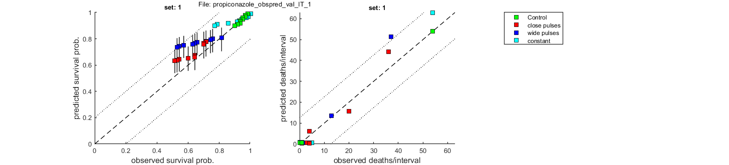
BLOCK 4. Validation: comparison to new data

The function [plot_main] can directly be used to make predictions (with CI) for new scenarios (not used for calibration) and compare them with data. As input, it needs a new data set, in the same way as for the calibration data set. This also implies that it is possible to use multiple data sets (although we allow only 1 for the standalone software). Optimised parameter values and confidence region will be read from a saved MAT file.

The data set is treated in the same manner as the calibration data. It is translated to the internal representation, which is returned in [data_val]. This definition is NOT made global; it is simply passed on to the plotting routine.

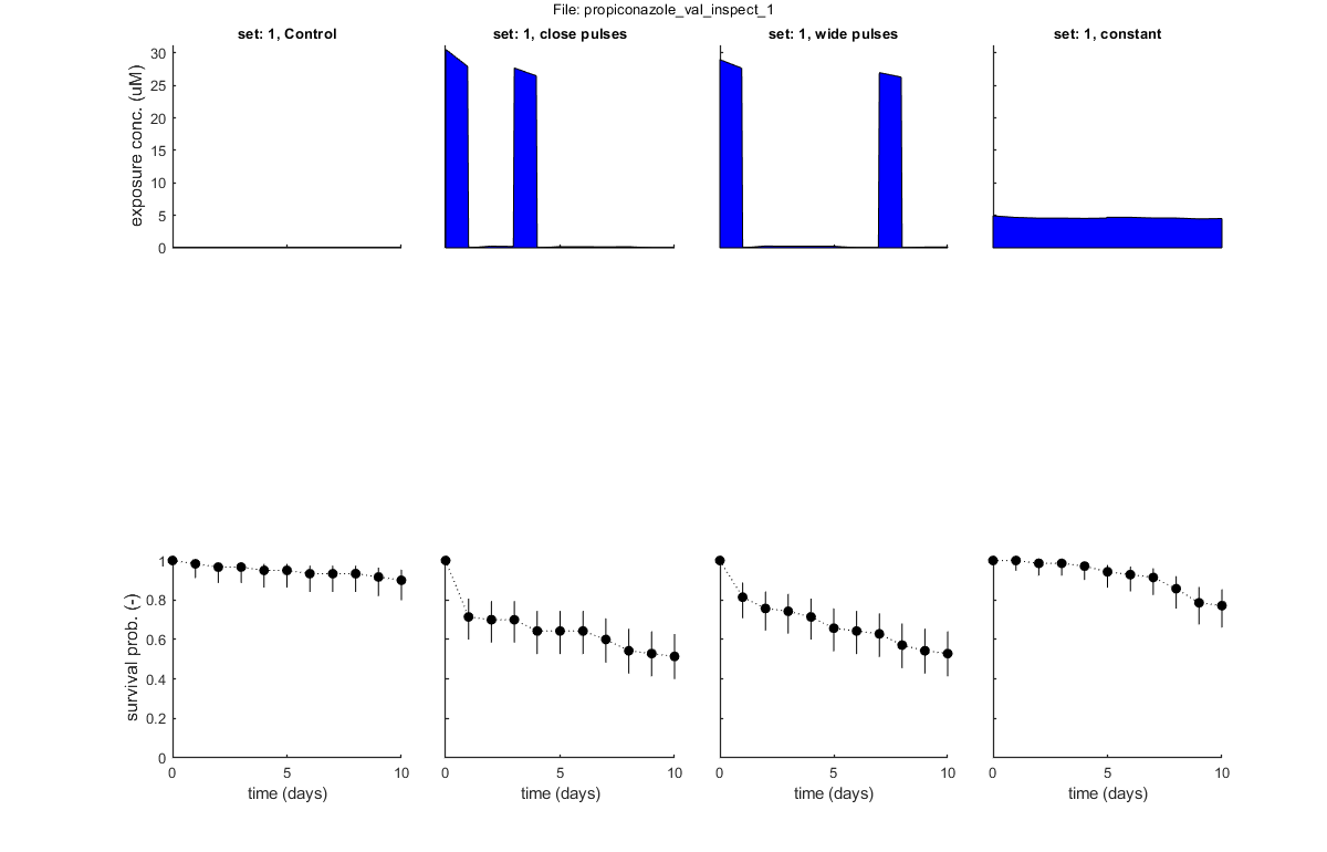
GLO.fix_hb_val = 1; % when set to 1, fit [hb] to the control data for all validation data sets, and keep fixed

% BLOCK 4.1. Load and prepare validation data.
[filename,filepath] = uigetfile('input_data/*.txt','Select file(s) for validation','MultiSelect','on'); % use Matlab GUI to select file(s)
if ~iscell(filename) && numel(filename) == 1 && filename(1) == 0 % if cancel is pressed ...
    return % simply stop
end

[data_val,error_flag] = load_data(filename,filepath,2); % load and prepare the data set for stage 2 (returned as structured cell array, so [data_all] can include multiple data sets)
if error_flag == 1 % see if there are errors spotted in the input file
    return % simply return (stop and do nothing)
end
plot_main(data_val,1,[2 0]) % inspection plot of data (stage 2, plot model off)
% Note: the 2 in the calls above signal that we are loading, preparing and
% plotting data for stage 2: validations.

% BLOCK 4.2. Call the plotting routine for validation plots (with model output).
plot_main(data_val,1,[2 1]) % SD validation: compare to model predictions (stage 2, plot model on)
plot_main(data_val,2,[2 1]) % IT validation: compare to model predictions (stage 2, plot model on)

% return % the return stops the analysis, so we can run this script in parts

Following data sets are loaded for validation:
    set: 1, file: propiconazole_pulsed_linear.txt

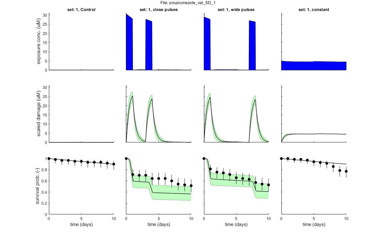
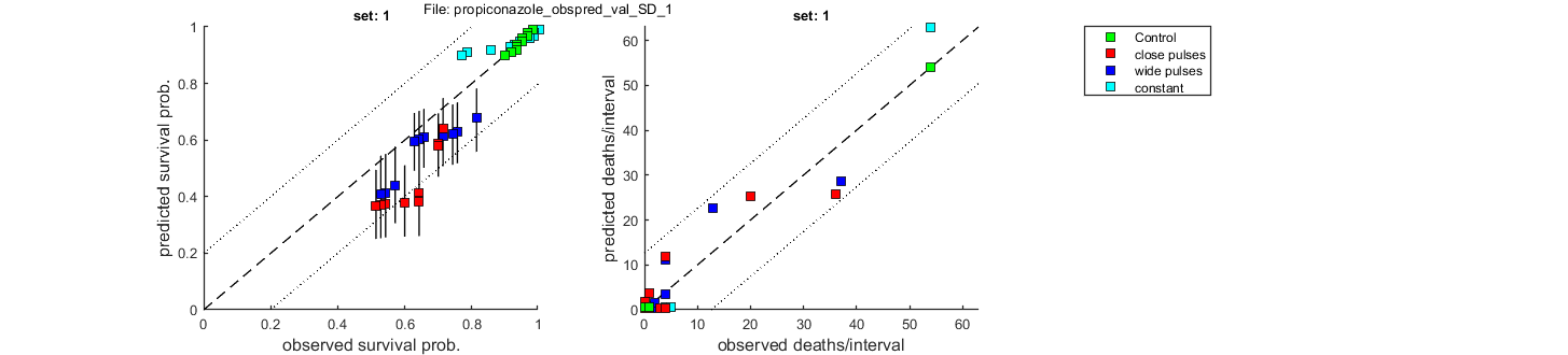
Goodness of fit measures for validation
  Special case: stochastic death (SD)
=====================================================================
Model efficiency (NSE, r-square)          : 0.5214 
Normalised root-means-square error (NRMSE): 14.822 % 
Survival probability prediction error (SPPE) for each treatment
     Data set     treatment    value
        1         Control     +0.00623 % 
        1      close pulses     +14.8 % 
        1      wide pulses     +11.9 % 
        1        constant     -12.9 % 
=====================================================================
Warning: these measures need to be interpreted more qualitatively
  as they, strictly speaking, do not apply to quantal data

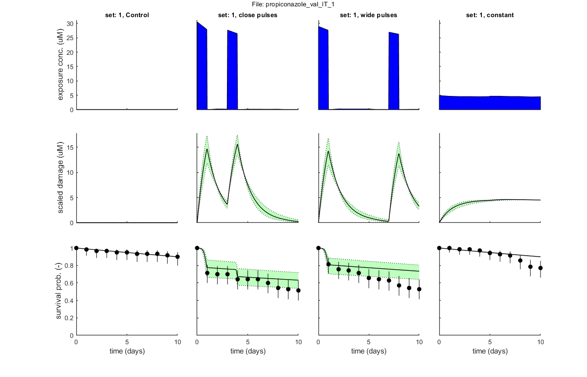
Goodness of fit measures for validation
  Special case: individual tolerance (IT)
=====================================================================
Model efficiency (NSE, r-square)          : 0.7504 
Normalised root-means-square error (NRMSE): 10.702 % 
Survival probability prediction error (SPPE) for each treatment
     Data set     treatment    value
        1         Control     +0.00623 % 
        1      close pulses     -11.8 % 
        1      wide pulses     -20.6 % 
        1        constant     -12.8 % 
=====================================================================
Warning: these measures need to be interpreted more qualitatively
  as they, strictly speaking, do not apply to quantal data

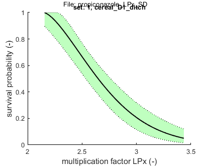
BLOCK 5. Predictions: LPx

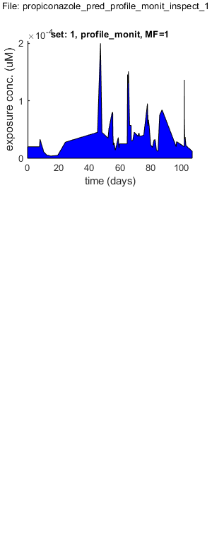
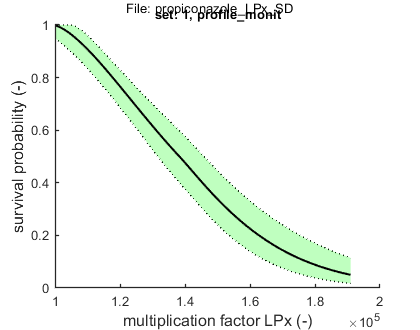
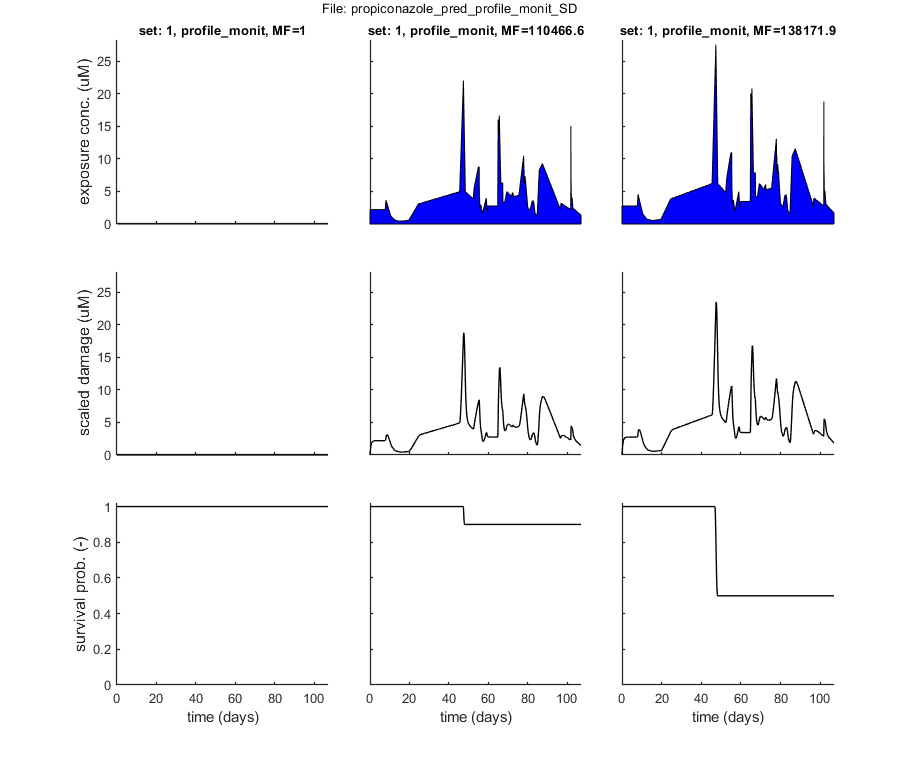
LPx is calculated for various effect levels (defined in [initial_setup]). This is the factor by which a given exposure scenario needs to be multiplied to result in x% mortality at the end of the profile, relative to the control. Optimised parameter values and confidence region will be read from the saved MAT file.

Exposure scenarios need to be entered as text files. However, only one treatment is allowed per data set. Multiple data sets can be used (although we allow only 1 for the standalone software). The scenario is thus a matrix with two columns: time (in days) and exposure concentration (in the same units as the data used for calibration!). This will be linearly interpolated.

Note: the second entry in the call to [calc_lpx] is a flag that is used for faster calculations (no CI) and batch processing. Note that flag setting 2 will probably not be used in the standalone software, but it is handy for testing (as CIs on LPx can take a very long calculation time). flag 1) regular, 2) no CI (very fast), 3) batch processing (no output to screen, no diary, no CIs)

% BLOCK 5.1. Load and prepare prediction data.
[filename,filepath] = uigetfile('input_profile/*.txt','Select file(s) with exposure profiles for standard predictions','MultiSelect','on'); % use Matlab GUI to select file(s)
if ~iscell(filename) && numel(filename) == 1 && filename(1) == 0 % if cancel is pressed ...
    return % simply stop
end

[data_pred,error_flag] = load_data(filename,filepath,3); % load and prepare the data set for stage 3 (returned as structured cell array, so [data_all] can include multiple data sets)
if error_flag == 1 % see if there are errors spotted in the input file
    return % simply return (stop and do nothing)
end
plot_main(data_pred,[],[3 0],[]) % inspection plot of data (stage 3, plot model off)
% Note: the 3 in the calls above signal that we are loading, preparing and
% plotting data for stage 3: predictions.

% BLOCK 5.2. Calculate LPx and plot.
sdit = 1; % select death mechanism: 1) SD 2) IT
LPx  = calc_lpx(data_pred,1,sdit); % calculates LPx values (1 with CI, 2 without) and makes a plot
plot_main(data_pred,sdit,[3 1],[ones(size(LPx,1),1) LPx]) % plot of data (stage 3, plot model on), pass on the calculated LPx values
% Note: by default, predictions are plotted without CIs. However, setting
% the flag in [plot_main] from [3 1] to [3 2] creates model curves *with*
% CIs (terribly slow for FOCUS profiles). Note: the vector
% [ones(size(LPx,1),1) LPx] in [calc_lpx] specifies which multiplication
% factors to use for plotting. I add the [ones] here to also plot the
% survival due to the unmodified exposure profile (as is also done in the
% standalone software).

% return % the return stops the analysis, so we can run this script in parts

Following exposure profiles are loaded for predictions:
    set: 1, file: profile_monit.txt

Results table for LPx (-) with 95% CI: profile_monit
  Special case: stochastic death (SD)
==================================================================
LPx     best       CI
==================================================================
LP10: 1.105e+05 (1.046e+05 - 1.146e+05)   
LP50: 1.382e+05 (1.315e+05 - 1.457e+05)   
==================================================================
Time required for the LPx calculations: 1 min, 30.7 secs

BLOCK 6. Batch predictions for LPx

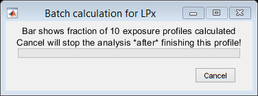
The function [calc_batch_lpx] can run a number of profiles sequentially, without output to screen (apart from a progress bar) until it is finished. The function returns the filename for the scenario that leads to the lowest (=worst) LP50 value (that could then be used for more detailed scrutiny). Plots for survical vs. time will appear in the directory [output_report], but not on screen.

Note that the call to [calc_batch_lpx] includes a correction factor [corr_factor] that can be used to correct for different units of the exposure profile, if needed. We decided not to use that for the software. Also note that the batch calculation can optionally be performed with CIs on the LPx values. This is also not part of the standalone. Calculations with CIs can be slow, so consider using a sub-sample from parameter space with [GLO.n_lim].

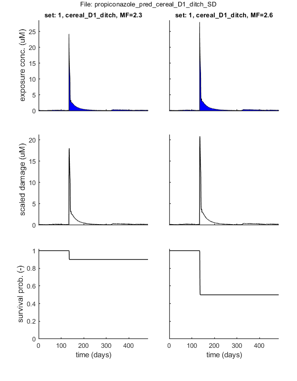
% BLOCK 6.1. Select files with exposure profiles for batch prediction.
[filename,filepath] = uigetfile('input_profile/*.txt','Select file(s) with exposure profiles for batch predictions','MultiSelect','on'); % use Matlab GUI to select file(s)
if ~iscell(filename) && numel(filename) == 1 && filename(1) == 0 % if cancel is pressed ...
    return % simply stop
end

% Note: the EFSA opinion also uses the propiconazole data set as a case
% study. However, there is some confusion regarding the concentration
% units. The calibration data are reported as nmol/ml (or uM) whereas the
% exposure profiles are in ug/L. These profiles are distributed on the
% openGUTS download page unchanged, to allow the users to reproduce the
% same numbers as in the opinion. Below, we can set a correction factor.
% However, these profiles are examples only, and not meant to be used for
% research or regulatory application.

corr_factor = 1; % to reconstruct the results in the EFSA opinion (and for the software, we don't use this correction factor)
% corr_factor = 1 / 342.2; % correction factor for ug/L (profiles) -> uM (calibration data)

% BLOCK 6.2. Run batch-calculation of all profiles and return worst one.
sdit       = 1; % select death mechanism: 1) SD 2) IT
GLO.n_lim  = [100]; % option to use random sub-sample of given size from the outer rim to speed things up (set empty [] to use full outer rim)
% Using a sub-sample increases speed, but underestimates the width of the
% CIs. How much it underestimates is difficult to say: it depends on the
% sampling, the parameter space, and on the exposure profile. In most
% cases, the difference for a sub-sample of 100 sets will be <5%. However,
% in one case of slow kinetics, and a profile with many peaks, I found a
% difference of 20%. Use with care.

% NOTE: the last flag in the call below is used to signal whether to do
% batch-calculation of LPx without (1) or with (2) CIs!
scen_worst = calc_batch_lpx(filename,filepath,sdit,corr_factor,1); % call [calc_batch_lpx] to do the calculations, and return name of worst profile

% return % the return stops the analysis, so we can run this script in parts

% BLOCK 6.3. Detailed analysis for the worst one from the batch calculations.
% Note: this is identical to the procedure in Block 5, but using the
% filename in [scen_worst] rather than selecting files with the Matlab GUI.
[data_pred,error_flag] = load_data(scen_worst,filepath,3,corr_factor); % load and prepare the data set for stage 3 (returned as structured cell array, so [data_all] can include multiple data sets)
if error_flag == 1 % see if there are errors spotted in the input file
    return % simply return (stop and do nothing)
end

LPx = calc_lpx(data_pred,1,sdit); % calculates LPx values (1 with CI, 2 without) (and makes a plot)
plot_main(data_pred,sdit,[3 1],LPx) % plot of data (stage 3, plot model on), pass on the calculated LPx values
% Note: by default, predictions are plotted without CIs. However, setting
% the flag in [plot_main] from [3 1] to [3 2] creates model curves *with*
% CIs (terribly slow for FOCUS profiles).

% return % the return stops the analysis, so we can run this script in parts

 
Starting batch processing ...

LPx values, scenarios ordered by descending risk (sorted on LP50)
  Special case: stochastic death (SD)
file analysed             LP10       LP50 
======================================================================================
cereal_D1_ditch           2.293      2.648 
cereal_D5_pond            11.04      11.65 
cereal_D4_pond            11.07      11.70 
cereal_D3_ditch           8.595      12.25 
apple_R1_pond             15.90      16.71 
cereal_D1_stream          13.62      20.23 
cereal_R4_stream          30.57      38.41 
apple_R2_stream           31.84      43.40 
cereal_D5_stream          113.6      193.3 
cereal_D4_stream          119.9      204.0 
======================================================================================
Following exposure profiles are loaded for predictions:
    set: 1, file: cereal_D1_ditch.txt
Results table for LPx (-) with 95% CI: cereal_D1_ditch
  Special case: stochastic death (SD)
==================================================================
LPx     best       CI
==================================================================
LP10: 2.293 (2.152 - 2.393)   
LP50: 2.648 (2.534 - 2.763)   
==================================================================
Time required for the LPx calculations: 30 mins, 33.0 secs

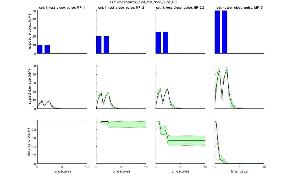
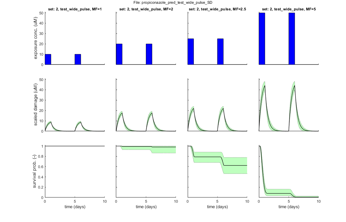
BLOCK 7. Demonstration of predictions for test design

The ability to make predictions can also be used for efficient test design. Here, an example is given. The user should prepare one or more scenarios of choice, e.g., with various pulses. With MF, the user can specify multiplication factors to plot, and [plot_main] will plot the associated damage and survival over time (here with CIs).

For testing, after calibration with propiconazole data for constant exposure, try the two test profiles in the directory [pulses_test_design]. These also work well with the dieldrin case study.

% BLOCK 7.1. Select file(s) with exposure profiles for prediction.
[filename,filepath] = uigetfile('input_profile/*.txt','Select file(s) with exposure profiles for test-design predictions','MultiSelect','on'); % use Matlab GUI to select file(s)
if ~iscell(filename) && numel(filename) == 1 && filename(1) == 0 % if cancel is pressed ...
    return % simply stop
end

[data_pred,error_flag] = load_data(filename,filepath,3); % load and prepare the data set for stage 3 (returned as structured cell array, so [data_all] can include multiple data sets)
if error_flag == 1 % see if there are errors spotted in the input file
    return % simply return (stop and do nothing)
end

% BLOCK 7.2. Plot predictions.
sdit = 1; % select death mechanism: 1) SD 2) IT
MF   = [1 2 2.5 5]; % these are the multiplication factors to plot
MF   = ones(data_pred.nr_sets,1) * MF; % make sure there is the same MF for all profiles that are entered

plot_main(data_pred,sdit,[3 2],MF) % plot of data (stage 3, plot model on), with the different MF values
% Note: the flag in [plot_main] of [3 2] creates model curves *with* CIs.

Following exposure profiles are loaded for predictions:
    set: 1, file: test_close_pulse.txt
    set: 2, file: test_wide_pulse.txt